Section: New Results
Image assimilation
Sequences of images, such as satellite acquisitions, display structures evolving in time. This information is recognized of major interest by forecasters (Meteorologists, oceanographers, etc) in order to improve the information provided by numerical models. However, these satellite images are mostly assimilated in geophysical models on a point-wise basis, discarding the space-time coherence visualized by the evolution of structures such as clouds. Assimilating in an optimal way image data is of major interest and this issue should be considered in two ways:
-
from the model's viewpoint, the problem is to control the location of structures using the observations,
-
from the image's viewpoint, a model of the dynamics and structures has to be built from the observations.
Divergence-free motion estimation
Participants : Dominique Béréziat [UPMC/LIP6] , Isabelle Herlin, Nicolas Mercier, Sergiy Zhuk.
This research addresses the issue of divergence-free motion estimation on an image sequence, acquired over a given temporal window. Unlike most state-of-the-art technics, which constrain the divergence to be small thanks to Tikhonov regularisation terms, a method that imposes a null value of divergence of the estimated motion is defined.
Motion is characterized by its vorticity value and assumed to satisfy the Lagragian constancy hypothesis. An image model is then defined: the state vector includes the vorticity, whose evolution equation is derived from that of motion, and a pseudo-image that is transported by motion. An image assimilation method, based on the 4D-Var technics, is defined and developed that estimates motion as a compromise between the evolution equations of vorticity and pseudo-image and the observed sequence of images: the pseudo-images have to be similar to the acquisitions.
As the evolution equations of vorticity and pseudo-image involve the motion value, the motion field has to be retrieved at each time step of the studied temporal window. An algebraic method, based on the projection of vorticity on a subspace of eigenvectors of the Laplace operator, is defined in order to allow Dirichlet boundary conditions for the vorticity field.
The divergence-free motion estimation method is tested and quantified on synthetic data. This shows that it computes a quasi-exact solution and outperforms the state-of-the-art methods that were applied on the same data.
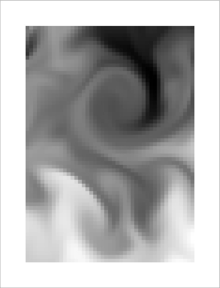
The method is also applied on Sea Surface Temperature (SST) images acquired over Black Sea by NOAA-AVHRR sensors. The divergence-free assumption is roughly valid on these acquisitions, due to the small values of vertical velocity at the surface. Fig. 5 displays data and results. As no ground truth of motion is available, the method is quantified by the value of correlation between the pseudo-images and the real acquisitions. Again, the method provides the best result compared to other state-of-the-art algorithms.


Improvement of motion estimation by assessing errors on the dynamics
Participants : Dominique Béréziat [UPMC/LIP6] , Isabelle Herlin, Nicolas Mercier.
Data assimilation technics are used to retrieve motion from image sequences. These methods require a model of the underlying dynamics, displayed by the evolution of image data. In order to quantify the approximation linked to the chosen dynamic model, we consider adding a model error term in the evolution equation of motion and design a weak formulation of 4D-Var data assimilation. The cost function to be minimized simultaneously depends on the initial motion field, at the begining of the studied temporal window, and on the error value at each time step. The result allows to assess the model error and analyze its impact on motion estimation.
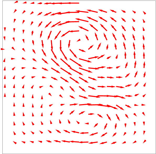
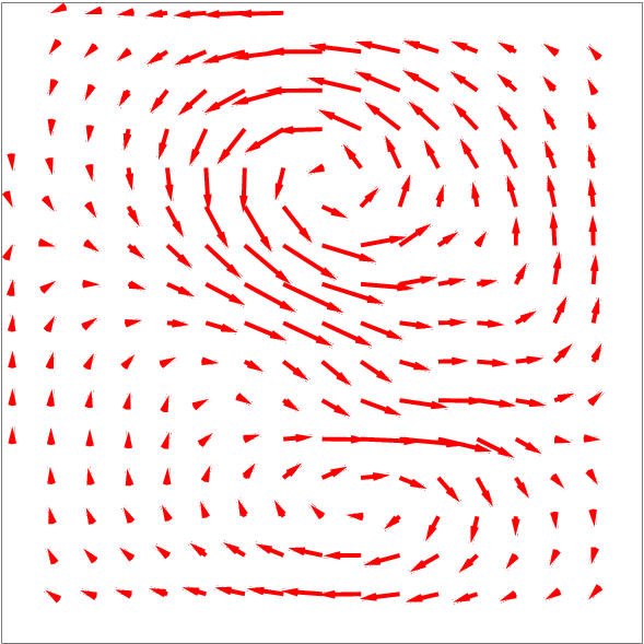
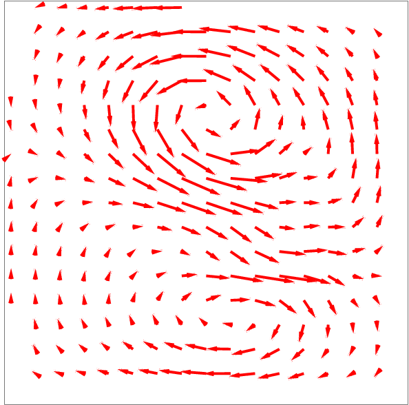
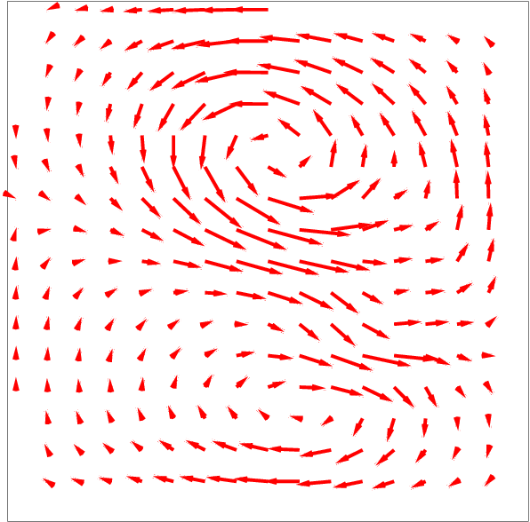
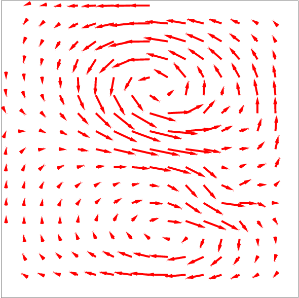
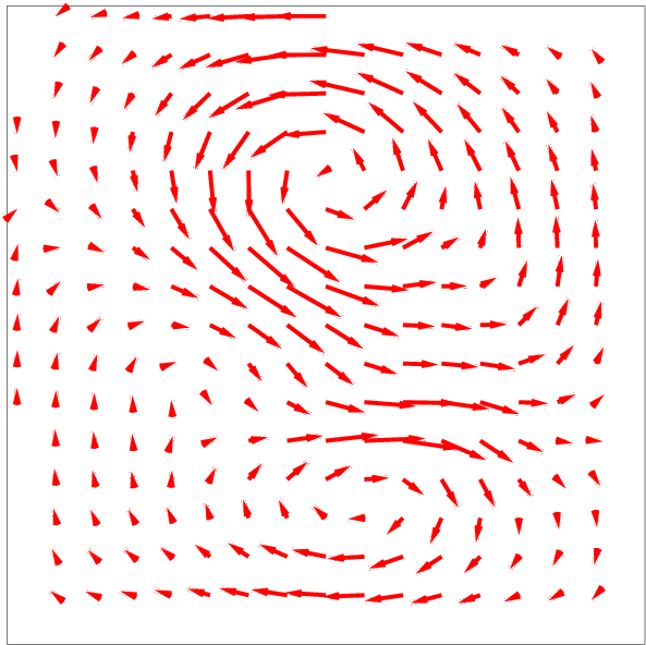
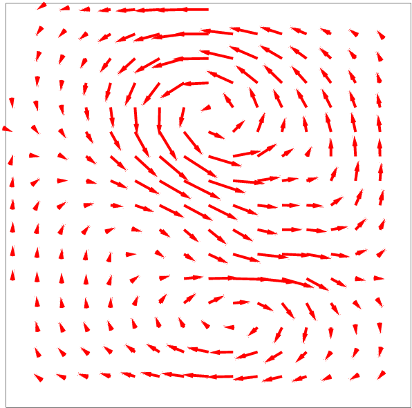
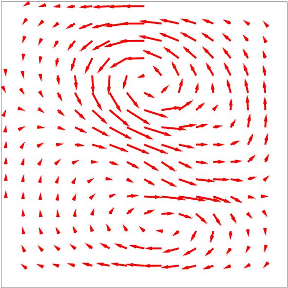
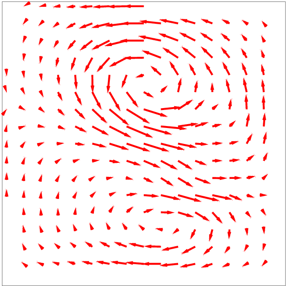
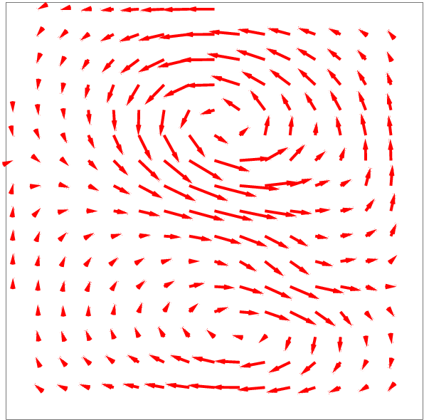
This error assessment method is evaluated and quantified on twin experiments, as no ground truth would be available for real image data. Fig. 6 shows four frames of a series of observations obtained by integrating the evolution model from an initial condition on image and velocity field (the ground truth displayed on the left of Fig. 7 ). An error value is added at each time step on the motion value, when integrating the simulation model. This error is a constant bias.

We performed two data assimilation experiments. The first one considers the evolution model as perfect, with no error in the evolution equation. It is denoted PM (for Perfect Model). The second one, denoted IM (for Imperfect Model) involves an error in the motion evolution equation. In fig.7 are displayed the motion fields retrieved by PM and IM at the beginning of the temporal window.
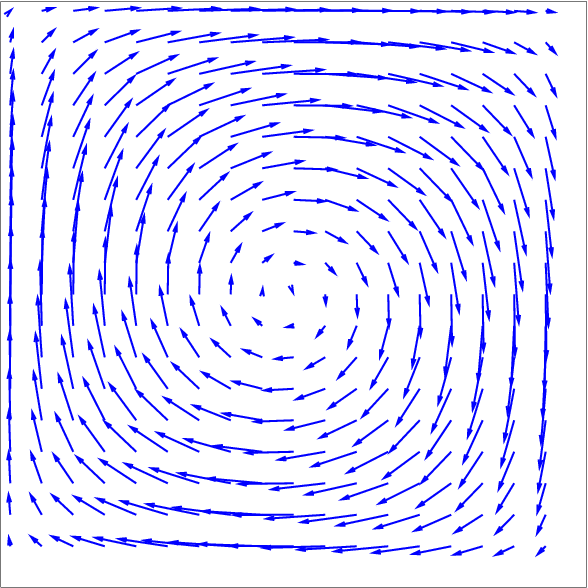
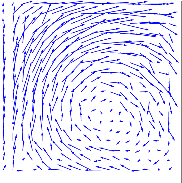
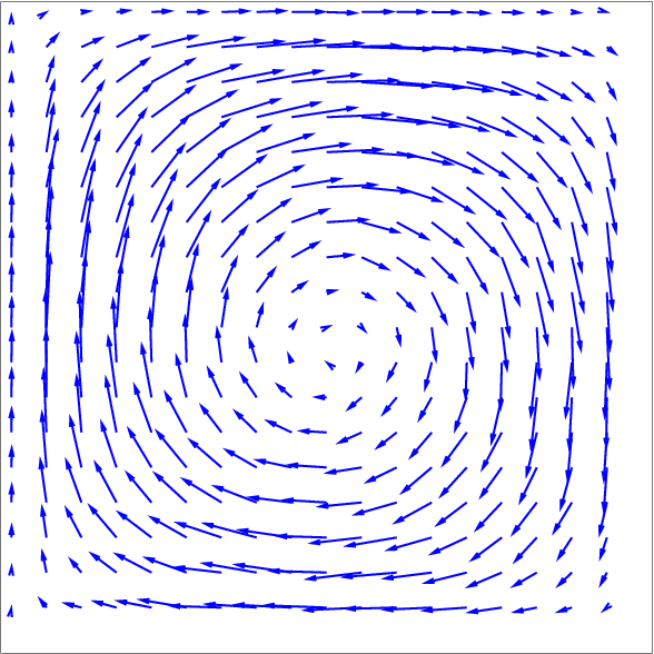
As it can be seen, IM computes a correct velocity field while PM completely fails.
The results on this error assessment method are still preliminary. Perspectives are considered in order to correctly retrieve the error on dynamics by constraining its shape. An important application is, for instance, the detection of dynamics changes on long temporal sequences.
Nonlinear Observation Equation For Motion Estimation
Participants : Dominique Béréziat [UPMC/LIP6] , Isabelle Herlin.
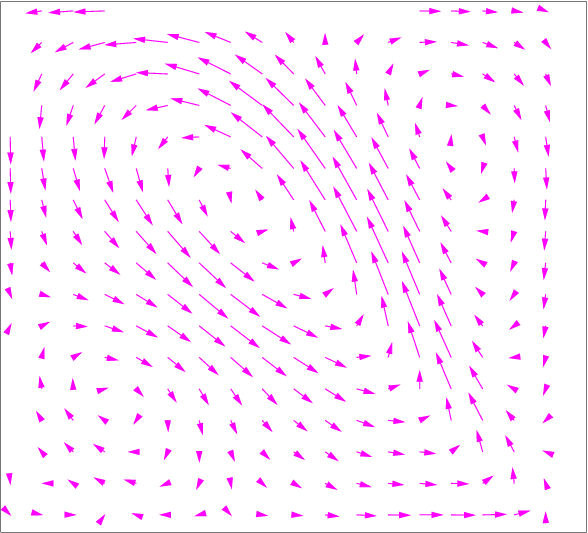
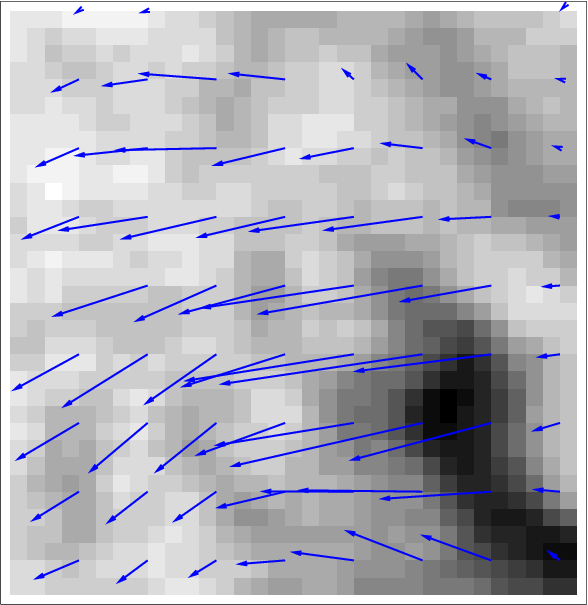
In the image processing literature, the optical flow equation is usually chosen to assess motion from an image sequence. However, it corresponds to an approximation that is no more valid in case of large displacements. We evaluate the improvements obtained when using the non linear transport equation of the image brightness by the velocity field. A 4D-Var data assimilation method is designed that simultaneously solves the evolution equation and the observation equation, in its non linear and linearized form. The comparison of results obtained with both observation equations is quantified on synthetic data and discussed on oceanographic Sea Surface Temperature (SST) images. We show that the non linear model outperforms the linear one, which underestimates the motion norm. Fig.8 illustrates this on SST images (motion vectors are displayed by arrows).
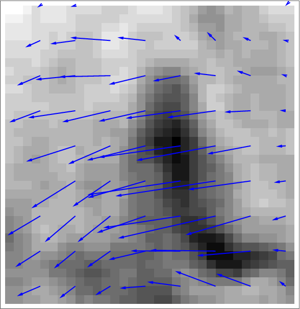
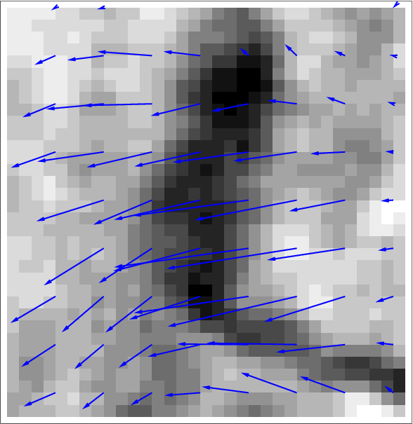
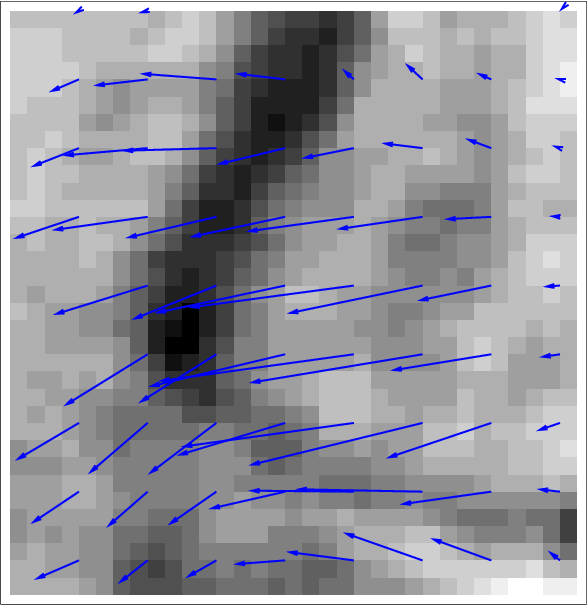
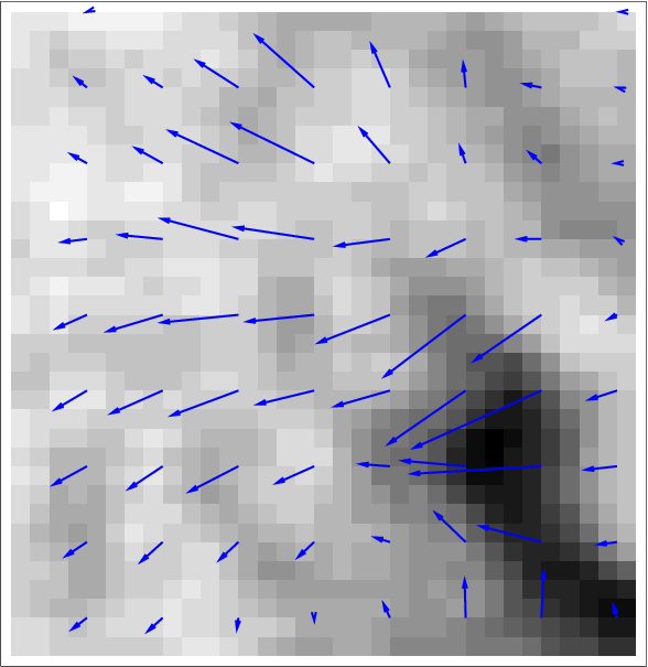
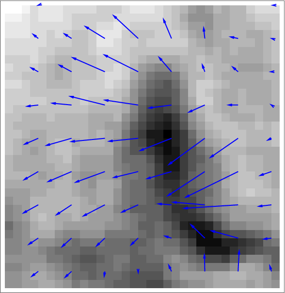
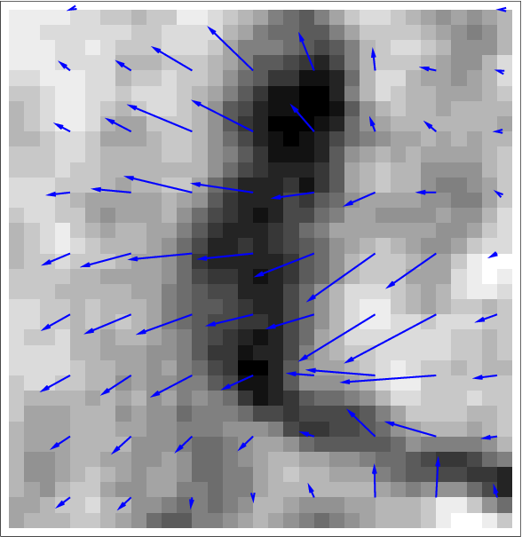
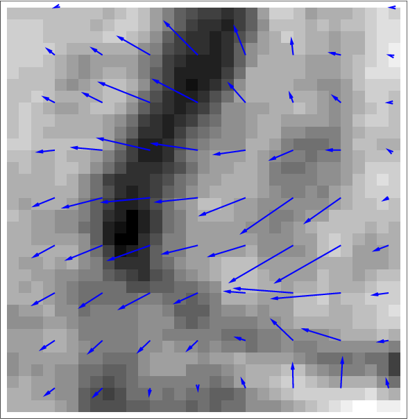
The aim of this research is to achieve a correct estimation of motion when the object displacement is greater than its size. In this case, coarse-to-fine incremental methods as well as the non linear data assimilation method fail to retrieve a correct value. The perspective is then to include, in the state vector, a variable describing the trajectory of pixels. The observation operator will then measure the effective displacement of pixels, according to their trajectories, and allow a better estimation of motion value.
Recovering missing data on images
Participants : Dominique Béréziat [UPMC/LIP6] , Isabelle Herlin, Nicolas Mercier.
A data assimilation method was designed to recover missing data and reduce noise on satellite acquisition. The state vector includes motion and image fields. Its evolution equation is based on assumptions on the underlying dynamics displayed by the sequence of images and considers the passive transport of images by the velocity field. The observation equation compares the image component of the state vector and the real observations. Missing and noisy data regions are characterized by a gaussian observation error, whose covariance matrix has an approximately infinitesimal inverse. The noise recovering method computes a solution of the state vector that is a compromise between the evolution equation and the observation equation. The image component of the solution satisfies the assumptions on the dynamics and is close to the real acquisition according to the covariance matrix . This image component provides the reconstruction of the noisy acquisitions.
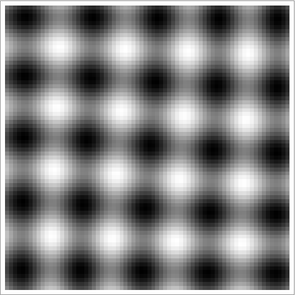
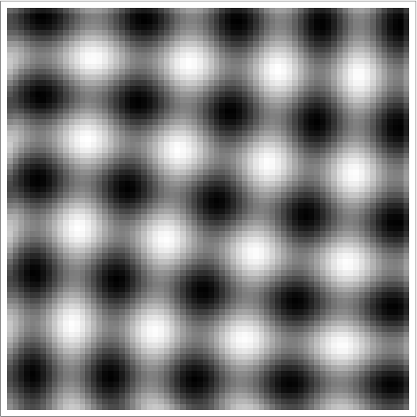
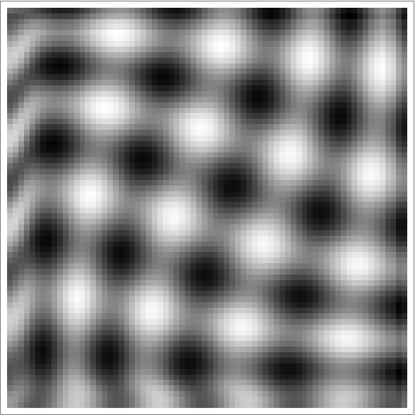
The recovering method was applied on synthetically noised SST images in order to quantify the quality of the recovering (see Fig.9 ).
|


The method is a promising alternative to those such as space-time interpolation. In the experiments, the Lagrangian constancy of the state vector is used as evolution equation. The perspectives concern the use of more advanced dynamic equations, as for instance the shallow water equations that link the motion field to the thickness of the ocean surface layer, and improved modeling of illumination changes over the sequence, due to various order acquisition times.
Validation of velocity estimated with image assimilation
Participants : Isabelle Herlin, Etienne Huot, Gennady Korotaev [Marine Hydrophysical Institute, Ukraine] , Evgeny Plotnikov [Marine Hydrophysical Institute, Ukraine] .
This study is achieved in collaboration with the Marine Hydrophysical Institute (MHI) of Sevastopol. The aim is to estimate and further validate the estimation of Black Sea surface velocity from sequences of satellite images in order to allow an optimal assimilation of these pseudo-observations in 3D ocean circulation models. Several Image Models were designed that express the dynamics of velocity and the temporal evolution of image data. An image assimilation method was developed based on the 4D-Var formalism and estimates motion as a compromise between the Image Model, the image acquisitions and regularity heuristics on the velocity field. Two Image Models were qualitatively and quantitatively compared: the Stationary Image Model (SIM) based on the heuristics of stationary motion, which is valid at short temporal scale, and the Shallow Water Image Model (SWIM), based on the shallow-water equations.
The comparison between SIM and SWIM results confirms that SIM provides correct results only on short temporal windows, while SWIM allows to process longer image sequences.
The validation of motion estimation by image assimilation requires additional observation data, as no measure of motion is available from satellite sensors. Sea Level Anomaly, measured by satellite altimeters, is then compared to the thickness of the surface layer as estimated by the Shallow Water Image Model. This comparison shows a good adequacy of shape and values [30] , [32] . As the velocity field is strongly related to this thickness value from the physical evolution laws, these results further validate the estimation of the velocity and the image assimilation approach.
Velocity estimation under the geostrophic equilibrium assumption
Participants : Isabelle Herlin, Etienne Huot.
The surface motion of the Black Sea approximately verifies the geostrophic equilibrium property. As the surface velocity can be directly derived from the surface layer thickness , this allows to simplify the shallow-water equations and the dynamics is expressed by the evolution of . The Geostrophic Shallow Water Image Model (GSWIM) is then designed based on the evolution of and the image data. A 4D-Var assimilation method was designed and developed in order to estimate from a sequence of satellite images. The motion field is then computed from the estimation of .
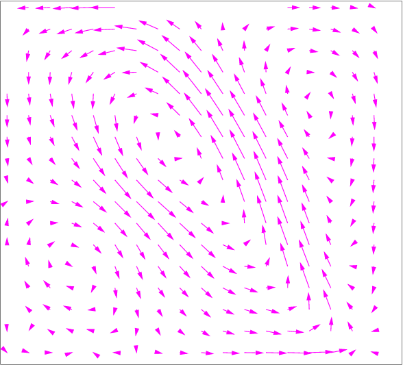
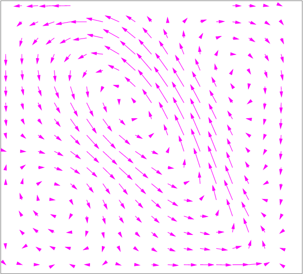
This method was first tested and quantified on twin experiments with satellite data. Figure 10 simultaneously displays the result of the velocity estimation by GSWIM and the ground truth.
|
Coupling models for motion estimation on long temporal image sequences
Participants : Karim Drifi, Isabelle Herlin.
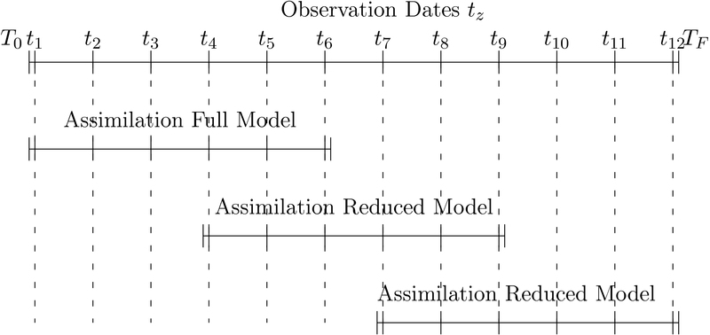
This study concerns the estimation of motion fields from satellite images on long temporal sequences. The huge computational cost and memory required by data assimilation methods on the pixel grid makes impossible to use these techniques on long temporal intervals. For a given dynamic model (named full model on the pixel grid), the Galerkin projection on a subspace provides a reduced model that allows image assimilation at low cost. The definition of this reduced model however requires defining the optimal subspace of motion. A sliding windows method is thus designed:
-
The long image sequence is split into small temporal windows that half overlap in time.
-
Data assimilation in the full model is applied on the first window to retrieve the motion field.
-
The estimate of motion field at the beginning of the second window makes it possible to define the subspace for motion and a reduced model is obtained by Galerkin projection.
-
Data assimilation in the reduced model is applied for this second window.
-
The process is then iterated for the next window until the end of the whole image sequence.
Figure 11 summarize the described methodology.
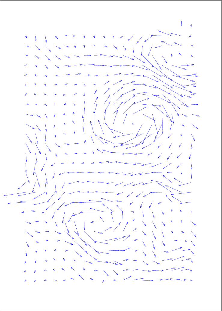
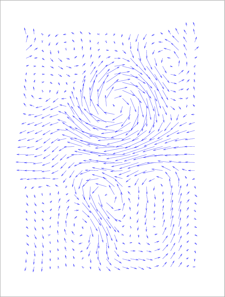
Twin experiments were designed to quantify the results of this sliding windows method. Results on motion estimation are given in Figure 12 and compared with the ground truth. The NRMSE (in percentage) ranges from 1.1 to 4.0% from the first to the sixth window. On the first window, 3 hours are required to estimate the motion fields with the full model. For the next 5 windows, less than 1 minute is required to compute motion.