Section: Application Domains

Introduction

We are working on problems that can be written in the following form

in a domain $\Omega \subset {ℝ}^d$, $d=1,2,3$, subjected to initial and boundary conditions. The variable $𝐔$ is a vector in general, the flux ${𝐅}_e$ is a tensor, as well as ${𝐅}_v$ which also depends on the gradient of $𝐔$. The subsystem

is assumed to be hyperbolic, the subsystem

is assumed to be elliptic. Last, (1 ) is supposed to satisfy an entropy inequality. The coefficients or models that define the flux and the boundary conditions can be deterministic or random.

The systems (1 ) are discretised mesh made of conformal elements. The tessalation is denoted by ${𝒯}_h$. The simplicies are denoted by $K_j$, $j=1,n_e$, and ${\cup }_j{K}_j={\Omega }_h$, an approximation of $\Omega$. The mesh is assumed to be adapted to the boundary conditions. In our methods, we assume a globaly continuous approximation of $𝐔$ such that ${𝐔}_{|K_j}$ is either a polynomial of degree $k$ or a more complex approximation such as a Nurbs. For now $k$ is uniform over the mesh, and let us denote by $V_h$ the vector space spanned by these functions, taking into account the boundary conditions.

The schemes we are working on have a variational formulation: find $𝐔\in V_h$ such that for any $𝐕\in V_h$,

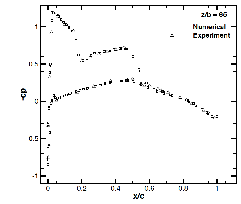
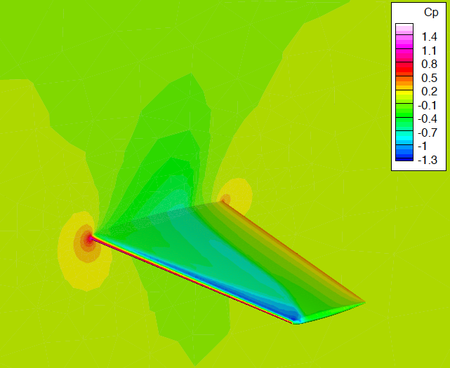
The variational operator $a(𝐔,𝐕;𝐖)$ is a sum of local operator that use onlty data within elements and boundary elements: it is very local. Boundary conditions can be implemented in a variational formulation or using a penalisation techbnique, see figure 1 . The third argument $𝐖$ stands for the way are implemented the non oscillatory properties of the method.

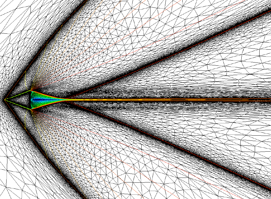
This leads to highly non linear systems to solve, we use typicaly non linear Krylov space techniques. The cost is reduced thanks to a parallel implementation, the domain is partionnned via Scotch . Mesh balancing, after mesh refinement, is handled via PaMPA . These schemes are implemented in RealfluiDS and, partialy, AeroSol . An example of such a simulation is given by Figure 2 .

In case of non determistic problems, we have a semi-intrusive strategy. The randomness is expressed via $N$ scalar random parameters (that might be correlated), $X=(x_1,...,x_N)$ with probability measure $d\mu$ which support is in a subset of ${ℝ}^N$. The idea of non intrusive methods is to approximate $d\mu$ either by $d\mu \approx {\sum }_j{\omega }_l{\delta }_{X_l}$ for ${\omega }_l\ge 0$ that sum up to unity, for “well chosen” samples $X_l$ or by $d\mu \approx {\sum }_l\mu \left({\Omega }_l\right)1_{X_j}dX$ where the sets ${\Omega }_j$ covers the support of $d\mu$ and are non overlapping.

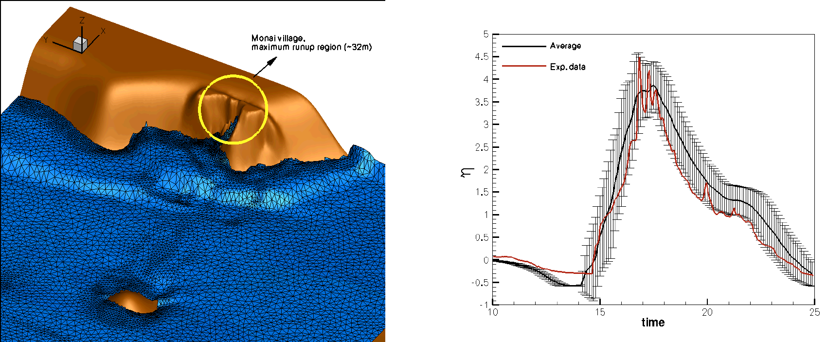
Staring from a discrete approximation of (1 ), we can implement randomess in the scheme. An example is given on figure 3 applied to the shallow water equations with dry shores, when the amplitude of the incoming tsunami wave is not known.