Section: New Results

Classification

Axon morphology comparison using elastic shape analysis

Participants : Alejandro Mottini, Xavier Descombes, Florence Besse.

It is known that neuronal morphology impacts network connectivity, thus providing information on its functioning. Moreover, it allows the characterization of pathological states. Therefore, the analysis of the morphological differences between normal and pathological structures is of paramount importance.

We present a new method for comparing reconstructions of axonal trees (obtained, for example, by applying our segmentation method on confocal microscopy images of normal and mutant axonal trees) which takes into account both topological and geometrical information and is based on the Elastic Shape Analysis Framework. The method computes the geodesic between two axons in a space of tree like shapes, and the distance between the two is defined as the length of the geodesic. Moreover, our method is capable of showing how one axon transforms into the other by taking intermediate points in the geodesic.

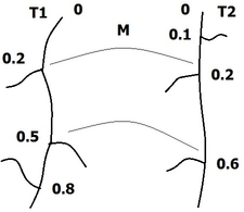
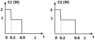
We consider two axonal trees $T_1$ and $T_2$, each consisting of an axon and several branches (and possibly sub branches). All are represented by 3D open curves in ${ℝ}^3$ (see Figure 10 ). We start by defining the matching function $M$ such that $M:(0,1,2,...n)\times (0,1,....,m)$, where $n$ and $m$ are the number of branches in $T_1$ and $T_2$ respectively. The matching function matches the branches of the two trees, for example, by assigning branch $i=1$ of $T_1$ to branch $j=3$ of $T_2$. We then define a branch function $C$ which indicates, for a given time $t_c$, how many branches remain after $\beta \left(t_c\right)$ (see Figure 10 ). We only take into account branches which have a match in the other axonal tree. Finally, we define the distance between two axonal trees $T_1,T_2$ as:

where ${\beta }_k$ is the main curve (axon) of tree $k$, $C_k$ its branch function, $M$ the matching function, ${\alpha }_{i,j}$ a weight parameter and $D(T_1\left(i\right),T_2\left(j\right))$ the distance between the matched branches of the two trees. All distances between simple curves are calculated using the elastic shape analysis framework.

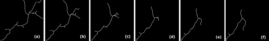
The method performance was tested on a group of 22 (11 normal and 11 mutant) 3D images, each containing one axonal tree manually segmented by an experienced biologist from a set of real confocal microscopy images. The mean and standard deviation of the inter and intra class distances between the neurons were calculated and results suggest that the proposed method is able to distinguish between the two populations (an average interpopulation to intrapopulation distance ratio of 1:21 and 1:28 were obtained). In addition, we computed the optimum transformations between axons. An example is shown in figure 11 . This result was obtained by taking intermediate points along the geodesic between the two trees.

Vascular network segmentation from X-ray tomographic volumes

Participant : Xavier Descombes.

This work was made in collaboration with Franck Plouraboué and Abdelakim El Boustani from IMFT, Caroline Fonta from CerCo, Géraldine LeDuc from ESRF, Raphael Serduc from INSERM and Tim Weitkamp from Synchrotron Soleil.

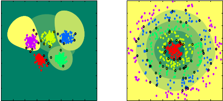
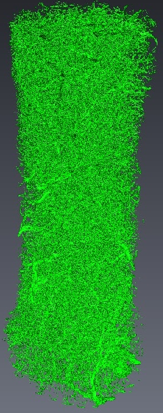
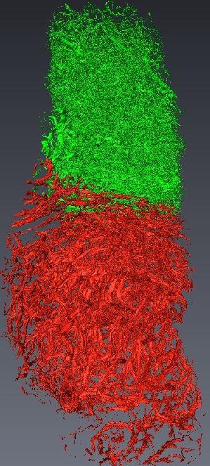
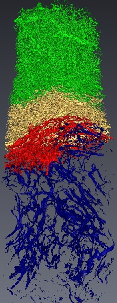
Micro-tomography produces high resolution images of biological structures such as vascular networks. We have defined a new approach for segmenting vascular network into pathological and normal regions from considering their micro-vessel 3D structure only. We consider a partition of the volume obtained by a watershed algorithm based on the distance from the nearest vessel. Each territory, defined as Local Vascular Territory (a Local Vascular Territory (LVT) is a connected region corresponding to the catchment bassin associated with a vascular element. It can be obtained through the watershed computation on the opposite distance map from the vessels and is not connected to the sample border. ), is characterized by its volume and the local vascular density. The volume and density maps are first regularized by minimizing the total variation, within a Markov Random Field framework, using a graph cut algorithm . Then, a new approach is proposed to segment the volume from the two previous restored images using an iterative algorithm based on hypothesis testing. We consider the variables density and volume for each LVT and the populations constituted by the different classes obtained by the segmentation at a given step. Classes which are not statistically significantly different are merged using a MANOVA. This blind segmentation provides different regions which have been interprated by expert as tumor, necrosis, tumor periphery and sane tissue 12 .

Statistical analysis of skin pigmentation under treatment

Participants : Sylvain Prigent, Xavier Descombes.

This work was partially funded by a contract with Galderma R&D [http://www.galderma.com/RampD.aspx ]. It was made in collaboration with J. Zerubia from Ayin team.

multispectral imaging, skin, hyperpigmentation, hypothesis tests, statistical inferences

One of the steps to evaluate the efficacy of a therapeutic solution is to test it on a clinical trial involving several populations of patients. Each population receives a studied treatment and a reference treatment for the disease.

For facial hyper-pigmentation, a group of $N_e$ patients receives the treatment on one cheek and a comparator on the other. The comparator can be a reference treatment or a placebo. To this end patients are selected to have the same hyper-pigmentation severity on the two cheeks. Then multi-spectral images are taken at different time $t$ along the treatment period.

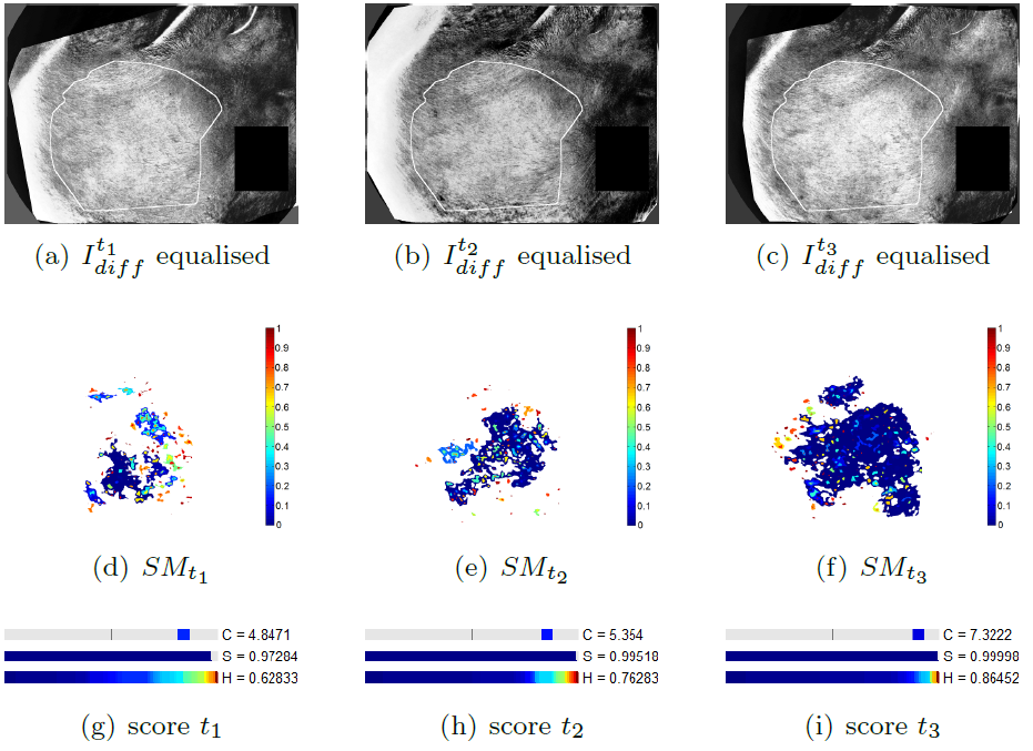
We propose a methodology to assess the efficacy a treatment by calculating three differential criteria: the darkness, the area and the homogeneity. The darkness measure the average intensity of the disease on a gray scaled image $I$ obtained by a linear combination of the spectral bands of the original multi-spectral image. A differential darkness is then obtained by measuring the deviation between the initial measurement at time $t_0$, and the measurement at time $t_k$. The differential area criterion is calculated by analyzing the histogram of $I_{diff}=I_{t_0}-I_{t_k}$ a difference gray scale image between two measurements in a time series. The differential homogeneity criterion is obtaining with a multi-scale analysis of $I_{diff}$ adapted from the Statistical Parametric Mapping (SPM) methodology. Indeed, statistical inferences allow to assign a probability of change to each region of $I_{diff}$ above a set of thresholds. These probabilities are calculated with respect to the maximum intensity and the spatial extend of each region. An integration of the obtained statistical map denoted $SM$, allows to get a homogeneity criterion.

The figure 13 illustrates the differential score calculated on a patient whose pathology decreases during the clinical trial. The proposed differential score have been tested in a full clinical study and provided results that agreed with the clinical analysis. This work have been patented and published in Inria research reports [25] , [26] .

A Recursive Approach For Multiclass Support Vector Machine: Application to automatic classification of endomicroscopic videos

Participants : Alexis Zubiolo, Eric Debreuve.

This work is made in collaboration with Barbara André (Mauna Kea Technologies)

The problem of automatic image (or video, or object) classification is to find a function that maps an image to a class or category among a number of predefined classes. An image can be viewed as a vector of high-dimension. In practice, it is preferable to deal with a synthetic signature of lower dimension. Therefore, the two classical steps of image classification are: image signature extraction and signature-based image classification. The classification rule can be learned from a set of training sample images manually classified by experts. This is known as supervised statistical learning where statistical refers to the use of samples and supervised refers to the sample classes being provided. We are interested in the learning aspect of the multiclass (Traditionally in classification, multiclass means “three classes or more” while the two-class case is referred to as binary classification.) problem when using a binary classification approach as a building block. We chose the Support Vector Machine (SVM), a well-known binary classifier.

Among the proposed extensions of binary classification methods to multiclass (three classes or more), the one-versus-one and one-versus-all approaches are the most popular ones. Let us suppose that there are $p\ge 3$ classes. The idea of the one-versus-all strategy is to oppose to any of the classes the union of the remaining $p-1$ classes. Then, $p$ SVM classifiers are determined, each one scoring, say, positively for one of the classes. The one-versus-one strategy opposes the classes by pair for all possible pairs. Therefore, $\frac{p(p-1)}{2}$ SVMs are determined and classification is performed by a majority vote.

As an alternative to these aforementioned strategies (as well as to other, less popular ones), we developed a recursive learning strategy. A tree of SVMs is built, achieving three goals: a fair balance in the number of samples used in each binary SVM learnings, a logarithmic complexity for classification (${log}_2\left(p\right)$ compared to the linear or quadratic complexities of one-versus-all or one-versus-one, respectively), and a coherent, incremental classification procedure (as opposed to selecting the final class based on possibly competing partial decisions). During learning, at each node of the tree, a combinatorial search is performed to determine an optimal separation of the current classification problem into two sub-problems. The proposed method was applied to automatic classification of endomicroscopic videos.